Quickstart
This guide will help you get up-and-running with crvUSDsim.
First, make sure that:
crvUSDsim is installed
crvUSDsim is up-to-date
Hello world
Before digging into more interesting examples, let’s check the installed package can run without issues. In the console, run:
$ python3 -m crvusdsim
[INFO][11:29:54][crvusdsim.pipelines.simple]-92751: Simulating mode: rate
[INFO][11:29:57][curvesim.price_data.sources]-92751: Fetching CoinGecko price data...
[INFO][11:30:08][curvesim.price_data.sources]-92751: Fetching CoinGecko price data...
[INFO][11:30:08][curvesim.price_data.sources]-92751: Fetching CoinGecko price data...
[INFO][11:30:08][curvesim.price_data.sources]-92751: Fetching CoinGecko price data...
[INFO][11:30:09][curvesim.price_data.sources]-92751: Fetching CoinGecko price data...
[INFO][11:30:16][crvusdsim.templates.Strategy]-92883: [Curve.fi Stablecoin wstETH] Simulating with {'rate0': 0.15}
[INFO][11:30:16][crvusdsim.templates.Strategy]-92880: [Curve.fi Stablecoin wstETH] Simulating with {'rate0': 0.1}
[INFO][11:30:16][crvusdsim.templates.Strategy]-92877: [Curve.fi Stablecoin wstETH] Simulating with {'rate0': 0.05}
Elapsed time: 28.6576099395752
Fetch a series of objects from Curve stablecoin wstETH market
Use collateral assets symbol, or if you know the address of the collateral asset, you can easily start interacting with it. crvUSDsim allows you to introspect on the market’s state and use its functions without submitting actual transactions on chain.
Begin by importing the crvUSDsim module:
>>> import crvusdsim
Let’s retrieve a series of objects from Curve stablecoin wstETH market:
>>> collateral_name = "wstETH" # or collateral_address "0x37417b2238aa52d0dd2d6252d989e728e8f706e4"
>>> (pool, controller, collateral_token, stablecoin, aggregator, stableswap_pools, peg_keepers, policy, factory)
>>>      = crvusdsim.pool.get(market_name)
Now, we have a series of wstETH market objects:
pool:SimLLAMMAPoolobjectcontroller:SimControllerobjectcollateral_token:ERC20objectstablecoin:StableCoinobjectaggregator:AggregateStablePriceobjectstableswap_pools: List[CurveStableSwapPool]peg_keepers: List[PegKeeper]policy:MonetaryPolicyobjectfactory:ControllerFactoryobject
Its state is pulled from daily snapshots of the Curve volume subgraph’s crvusd module. From this object we can retrieve state information and see the result of pool operations such as swaps or adding liquidity.
The pool interface adheres closely to the live smart contract’s, so if you are familiar with the vyper contract, you should feel at home.
For example, to check various data about the pool:
>>> pool.name
'Curve.fi Stablecoin wstETH'

>>> pool.coin_names
['wstETH', 'crvUSD']
>>> pool.A
100

>>> controller.loan_discount
90000000000000000

>>> controller.liquidation_discount
60000000000000000
Do some trade on pool, trade function will use ARBITRAGUR as trader’s address, and mint token to ARBITRAGUR automatically:
>>> dx = 10**18
>>> pool.trade(0, 1, dx) # dx, dy, fees
(1000000000000000000, 445225238462727, 6000000000000000)
If you want to dig into the pulled data that was used to construct the pool:
>>> pool.metadata
{'llamma_params': {'name': 'Curve.fi Stablecoin wstETH',
'address': '0x37417b2238aa52d0dd2d6252d989e728e8f706e4',
'A': '100',
'rate': '4010591623',
'rate_mul': '1024868101325770634',
'fee': '0.006',
'admin_fee': '0.000000000000000001',
'BASE_PRICE': '2117.144587304125327462',
'active_band': '-12',
'min_band': '-14',
'max_band': '1034',
'oracle_price': '2373.921229194305616293',
'collateral_address': '0x7f39c581f595b53c5cb19bd0b3f8da6c935e2ca0',
'collateral_precision': '18',
'collateral_name': 'wstETH',
'collateral_symbol': 'wstETH',
'bands_x': defaultdict(int,
   ...
'addresses': ['0xf939e0a03fb07f59a73314e73794be0e57ac1b4e', '0x7f39C581F595B53c5cb19bD0b3f8dA6c935E2Ca0'],
'decimals': [18, 18]},
'address': '0x37417b2238aa52d0dd2d6252d989e728e8f706e4',
'chain': 'mainnet'}
If you want to get objects with bands data or users’ loan data, simply use bands_data parameter, the valid value is pool or controller:
# get pool with `bands_x` and `bands_y` data
>>> (pool, controller, ...) = crvusdsim.pool.get(market_name, bands_data="pool")

>>> sum(pool.bands_x.values())
0
>>> sum(pool.bands_y.values())
40106052164494685140992

# get pool with `bands_x`, `bands_y`, `user_shares` data
# and controller with `loan`, `loans`, `loan_ix` data
>>> (pool, controller, ...) = crvusdsim.pool.get(market_name, bands_data="controller")

>>> len(pool.user_shares)
392

>>> len(controller.loan)
392

>>> user0 = controller.loans[1] # user address
>>> loan0 = controller.loan[user0] # :class:Loan
>>> (loan0.initial_debt, loan0.initial_collateral, loan0.rate_mul, loan0.timestamp)
(9779961749290509154648064, 6785745612366175797248, 1000000000000000000, 1700712599)
Run an arbitrage simulation for a proposed parameter
Rate simulations to see results of varying rate0 parameters in MonetaryPolicy:
>>> import crvusdsim
>>> res = crvusdsim.autosim(pool="wstETH", sim_mode="rate", rate0=[0.05, 0.075, 0.10, 0.125, 0.15])
[INFO][10:02:42][crvusdsim.pipelines.simple]-84886: Simulating mode: rate
[INFO][10:02:50][curvesim.price_data.sources]-84886: Fetching CoinGecko price data...
[INFO][10:03:51][curvesim.price_data.sources]-84886: Fetching CoinGecko price data...
[INFO][10:03:52][curvesim.price_data.sources]-84886: Fetching CoinGecko price data...
[INFO][10:05:44][curvesim.price_data.sources]-84886: Fetching CoinGecko price data...
[INFO][10:07:22][curvesim.price_data.sources]-84886: Fetching CoinGecko price data...
[INFO][10:07:32][crvusdsim.templates.Strategy]-84936: [Curve.fi Stablecoin wstETH] Simulating with {'rate0': 0.05}
[INFO][10:07:32][crvusdsim.templates.Strategy]-84937: [Curve.fi Stablecoin wstETH] Simulating with {'rate0': 0.125}
[INFO][10:07:32][crvusdsim.templates.Strategy]-84935: [Curve.fi Stablecoin wstETH] Simulating with {'rate0': 0.075}
[INFO][10:07:32][crvusdsim.templates.Strategy]-84934: [Curve.fi Stablecoin wstETH] Simulating with {'rate0': 0.1}
[INFO][10:07:33][crvusdsim.templates.Strategy]-84938: [Curve.fi Stablecoin wstETH] Simulating with {'rate0': 0.15}
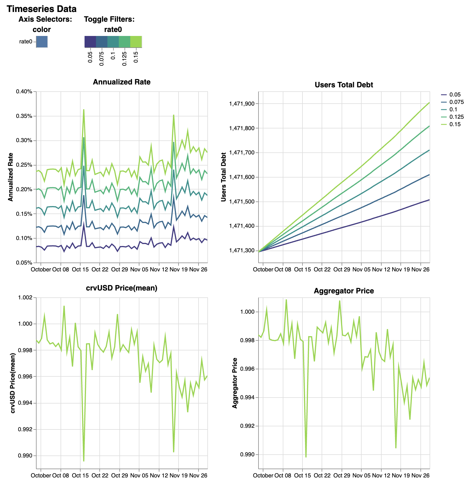
>>> res.summary()
metric annualized_rate users_debt crvusd_price agg_price
stat mean mean mean mean
0 0.000868 1.471397e+06 0.997661 0.997426
1 0.001287 1.471446e+06 0.997661 0.997426
2 0.001697 1.471495e+06 0.997661 0.997426
3 0.002097 1.471543e+06 0.997661 0.997426
4 0.002490 1.471589e+06 0.997661 0.997426
>>> res.summary(full=True)
rate0 annualized_rate mean users_debt mean crvusd_price mean agg_price mean
0 0.050 0.000868 1.471397e+06 0.997661 0.997426
1 0.075 0.001287 1.471446e+06 0.997661 0.997426
2 0.100 0.001697 1.471495e+06 0.997661 0.997426
3 0.125 0.002097 1.471543e+06 0.997661 0.997426
4 0.150 0.002490 1.471589e+06 0.997661 0.997426
>>> res.data()
run timestamp annualized_rate users_debt crvusd_price agg_price
0 0 2023-09-29 23:30:00+00:00 0.000824 1.471293e+06 0.998771 0.998381
1 0 2023-09-29 23:38:34+00:00 0.000824 1.471293e+06 0.998771 0.998381
2 0 2023-09-29 23:47:08+00:00 0.000824 1.471293e+06 0.998771 0.998381
3 0 2023-09-29 23:55:42+00:00 0.000824 1.471293e+06 0.998771 0.998381
4 0 2023-09-30 00:04:17+00:00 0.000824 1.471293e+06 0.998771 0.998381
... ... ... ... ... ... ...
51240 4 2023-11-29 22:55:42+00:00 0.002746 1.471905e+06 0.996052 0.995404
51241 4 2023-11-29 23:04:17+00:00 0.002746 1.471905e+06 0.996052 0.995404
51242 4 2023-11-29 23:12:51+00:00 0.002746 1.471905e+06 0.996052 0.995404
51243 4 2023-11-29 23:21:25+00:00 0.002746 1.471905e+06 0.996052 0.995404
51244 4 2023-11-29 23:30:00+00:00 0.002750 1.471905e+06 0.996052 0.995373
51245 rows x 6 columns
>>> res.data(full=True)
rate0 run timestamp annualized_rate users_debt crvusd_price agg_price
0 0.05 0 2023-09-29 23:30:00+00:00 0.000824 1.471293e+06 0.998771 0.998381
1 0.05 0 2023-09-29 23:38:34+00:00 0.000824 1.471293e+06 0.998771 0.998381
2 0.05 0 2023-09-29 23:47:08+00:00 0.000824 1.471293e+06 0.998771 0.998381
3 0.05 0 2023-09-29 23:55:42+00:00 0.000824 1.471293e+06 0.998771 0.998381
4 0.05 0 2023-09-30 00:04:17+00:00 0.000824 1.471293e+06 0.998771 0.998381
... ... ... ... ... ... ... ...
51240 0.15 4 2023-11-29 22:55:42+00:00 0.002746 1.471905e+06 0.996052 0.995404
51241 0.15 4 2023-11-29 23:04:17+00:00 0.002746 1.471905e+06 0.996052 0.995404
51242 0.15 4 2023-11-29 23:12:51+00:00 0.002746 1.471905e+06 0.996052 0.995404
51243 0.15 4 2023-11-29 23:21:25+00:00 0.002746 1.471905e+06 0.996052 0.995404
51244 0.15 4 2023-11-29 23:30:00+00:00 0.002750 1.471905e+06 0.996052 0.995373
51245 rows x 7 columns
Tuning a pool parameter, such as the amplification coefficient A.:
>>> import crvusdsim
>>> market_name = "wstETH"
>>> res = crvusdsim.autosim(pool="wstETH", sim_mode="pool", A=100)
[INFO][14:57:58][crvusdsim.pipelines.simple]-82656: Simulating mode: pool
[INFO][14:58:00][curvesim.price_data.sources]-82656: Fetching CoinGecko price data...
[INFO][14:58:05][crvusdsim.templates.Strategy]-82730: [Curve.fi Stablecoin wstETH] Simulating with {'A': 100}
Likely you will want to see the impact over a range of A values. The A and fee parameters
will accept either a integer or iterables of integers; note fee values are in units of basis points
multiplied by 10**18.:
>>> res = crvusdsim.autosim(pool="wstETH", sim_mode="pool", A=[50, 60, 80, 100], fee=[6 * 10**15, 10 * 10**15])

[INFO][11:08:46][crvusdsim.pipelines.simple]-33804: Simulating mode: pool
[INFO][11:09:10][curvesim.price_data.sources]-33804: Fetching CoinGecko price data...
[INFO][11:09:44][crvusdsim.templates.Strategy]-33869: [Curve.fi Stablecoin wstETH] Simulating with {'A': 50, 'fee': 6000000000000000}
[INFO][11:09:44][crvusdsim.templates.Strategy]-33870: [Curve.fi Stablecoin wstETH] Simulating with {'A': 50, 'fee': 10000000000000000}
[INFO][11:09:44][crvusdsim.templates.Strategy]-33876: [Curve.fi Stablecoin wstETH] Simulating with {'A': 60, 'fee': 10000000000000000}
[INFO][11:09:44][crvusdsim.templates.Strategy]-33875: [Curve.fi Stablecoin wstETH] Simulating with {'A': 100, 'fee': 6000000000000000}
[INFO][11:09:44][crvusdsim.templates.Strategy]-33873: [Curve.fi Stablecoin wstETH] Simulating with {'A': 80, 'fee': 6000000000000000}
[INFO][11:09:44][crvusdsim.templates.Strategy]-33871: [Curve.fi Stablecoin wstETH] Simulating with {'A': 60, 'fee': 6000000000000000}
[INFO][11:09:44][crvusdsim.templates.Strategy]-33872: [Curve.fi Stablecoin wstETH] Simulating with {'A': 80, 'fee': 10000000000000000}
[INFO][11:09:45][crvusdsim.templates.Strategy]-33874: [Curve.fi Stablecoin wstETH] Simulating with {'A': 100, 'fee': 10000000000000000}

>>> res.summary()

metric      pool_value      loss_value      pool_volume     arb_profit      pool_fees
stat        annualized_returns      annualized_arb_profits  sum     sum     sum
0   0.569850        0.031372        5.521713e+09    1.017937e+07    7.298168e+07
1   0.533898        0.025810        4.358760e+09    8.319915e+06    9.826156e+07
2   0.573620        0.029282        5.347932e+09    9.473498e+06    7.089184e+07
3   0.553401        0.022987        3.987458e+09    7.478085e+06    9.083868e+07
4   0.571523        0.029660        5.389022e+09    9.611733e+06    7.140822e+07
5   0.529070        0.027319        4.241904e+09    8.805979e+06    9.597500e+07
6   0.569426        0.030513        5.393248e+09    9.903716e+06    7.147705e+07
7   0.554593        0.022389        4.017923e+09    7.283106e+06    9.152026e+07

>>> res.summary(full=True)

    A       Fee     pool_value annualized_returns   loss_value annualized_arb_profits       pool_volume sum arb_profit sum  pool_fees sum
0   50      0.006   0.569850        0.031372        5.521713e+09    1.017937e+07    7.298168e+07
1   50      0.010   0.533898        0.025810        4.358760e+09    8.319915e+06    9.826156e+07
2   60      0.006   0.573620        0.029282        5.347932e+09    9.473498e+06    7.089184e+07
3   60      0.010   0.553401        0.022987        3.987458e+09    7.478085e+06    9.083868e+07
4   80      0.006   0.571523        0.029660        5.389022e+09    9.611733e+06    7.140822e+07
5   80      0.010   0.529070        0.027319        4.241904e+09    8.805979e+06    9.597500e+07
6   100     0.006   0.569426        0.030513        5.393248e+09    9.903716e+06    7.147705e+07
7   100     0.010   0.554593        0.022389        4.017923e+09    7.283106e+06    9.152026e+07

>>> res.data()

    run     timestamp       pool_value      loss_value      pool_volume     arb_profit      pool_fees
0   0       2023-09-29 23:30:00+00:00       1.879406e+09    0.000000        0.0     0.0     0.0
1   0       2023-09-29 23:38:34+00:00       1.879531e+09    0.000000        0.0     0.0     0.0
2   0       2023-09-29 23:47:08+00:00       1.879656e+09    0.000000        0.0     0.0     0.0
3   0       2023-09-29 23:55:42+00:00       1.879781e+09    0.000000        0.0     0.0     0.0
4   0       2023-09-30 00:04:17+00:00       1.879906e+09    0.000000        0.0     0.0     0.0
... ...     ...     ...     ...     ...     ...     ...
81987       7       2023-11-29 22:55:42+00:00       2.034973e+09    0.003707        0.0     0.0     0.0
81988       7       2023-11-29 23:04:17+00:00       2.034973e+09    0.003707        0.0     0.0     0.0
81989       7       2023-11-29 23:12:51+00:00       2.034973e+09    0.003707        0.0     0.0     0.0
81990       7       2023-11-29 23:21:25+00:00       2.034973e+09    0.003707        0.0     0.0     0.0
81991       7       2023-11-29 23:30:00+00:00       2.034973e+09    0.003707        0.0     0.0     0.0
81992 rows × 7 columns

>>> res.data(full=True)

            A       Fee     run     timestamp       pool_value      loss_value      pool_volume     arb_profit      pool_fees
0   50      0.006   0       2023-09-29 23:30:00+00:00       1.879406e+09    0.000000        0.0     0.0     0.0
1   50      0.006   0       2023-09-29 23:38:34+00:00       1.879531e+09    0.000000        0.0     0.0     0.0
2   50      0.006   0       2023-09-29 23:47:08+00:00       1.879656e+09    0.000000        0.0     0.0     0.0
3   50      0.006   0       2023-09-29 23:55:42+00:00       1.879781e+09    0.000000        0.0     0.0     0.0
4   50      0.006   0       2023-09-30 00:04:17+00:00       1.879906e+09    0.000000        0.0     0.0     0.0
... ...     ...     ...     ...     ...     ...     ...     ...     ...
81987       100     0.010   7       2023-11-29 22:55:42+00:00       2.034973e+09    0.003707        0.0     0.0     0.0
81988       100     0.010   7       2023-11-29 23:04:17+00:00       2.034973e+09    0.003707        0.0     0.0     0.0
81989       100     0.010   7       2023-11-29 23:12:51+00:00       2.034973e+09    0.003707        0.0     0.0     0.0
81990       100     0.010   7       2023-11-29 23:21:25+00:00       2.034973e+09    0.003707        0.0     0.0     0.0
81991       100     0.010   7       2023-11-29 23:30:00+00:00       2.034973e+09    0.003707        0.0     0.0     0.0
81992 rows x 9 columns
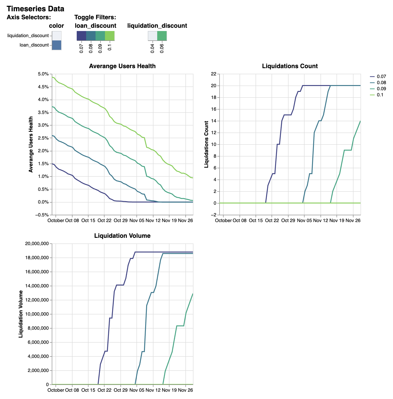
To simlate controller’s parameters, such as loan_discount and liquidation_discount, use sim_mode="controller":
>>> res = crvusdsim.autosim(pool="wstETH", sim_mode="controller",
>>> loan_discount=[int(0.07 * 10**18), int(0.08 * 10**18), int(0.09 * 10**18), int(0.10 * 10**18)],
>>> liquidation_discount=[int(0.04 * 10**18), int(0.06 * 10**18)])
[INFO][14:56:36][crvusdsim.pipelines.simple]-7441: Simulating mode: controller
[INFO][14:56:36][curvesim.price_data.sources]-7441: Fetching CoinGecko price data...
[INFO][14:57:15][crvusdsim.templates.Strategy]-41713: [Curve.fi Stablecoin wstETH] Simulating with {'loan_discount': 80000000000000000, 'liquidation_discount': 60000000000000000}
[INFO][14:57:16][crvusdsim.templates.Strategy]-41710: [Curve.fi Stablecoin wstETH] Simulating with {'loan_discount': 70000000000000008, 'liquidation_discount': 40000000000000000}
[INFO][14:57:16][crvusdsim.templates.Strategy]-41712: [Curve.fi Stablecoin wstETH] Simulating with {'loan_discount': 80000000000000000, 'liquidation_discount': 40000000000000000}
[INFO][14:57:16][crvusdsim.templates.Strategy]-41714: [Curve.fi Stablecoin wstETH] Simulating with {'loan_discount': 90000000000000000, 'liquidation_discount': 40000000000000000}
[INFO][14:57:16][crvusdsim.templates.Strategy]-41711: [Curve.fi Stablecoin wstETH] Simulating with {'loan_discount': 70000000000000008, 'liquidation_discount': 60000000000000000}
[INFO][14:57:16][crvusdsim.templates.Strategy]-41716: [Curve.fi Stablecoin wstETH] Simulating with {'loan_discount': 90000000000000000, 'liquidation_discount': 60000000000000000}
[INFO][14:57:16][crvusdsim.templates.Strategy]-41717: [Curve.fi Stablecoin wstETH] Simulating with {'loan_discount': 100000000000000000, 'liquidation_discount': 60000000000000000}
[INFO][14:57:16][crvusdsim.templates.Strategy]-41715: [Curve.fi Stablecoin wstETH] Simulating with {'loan_discount': 100000000000000000, 'liquidation_discount': 40000000000000000}
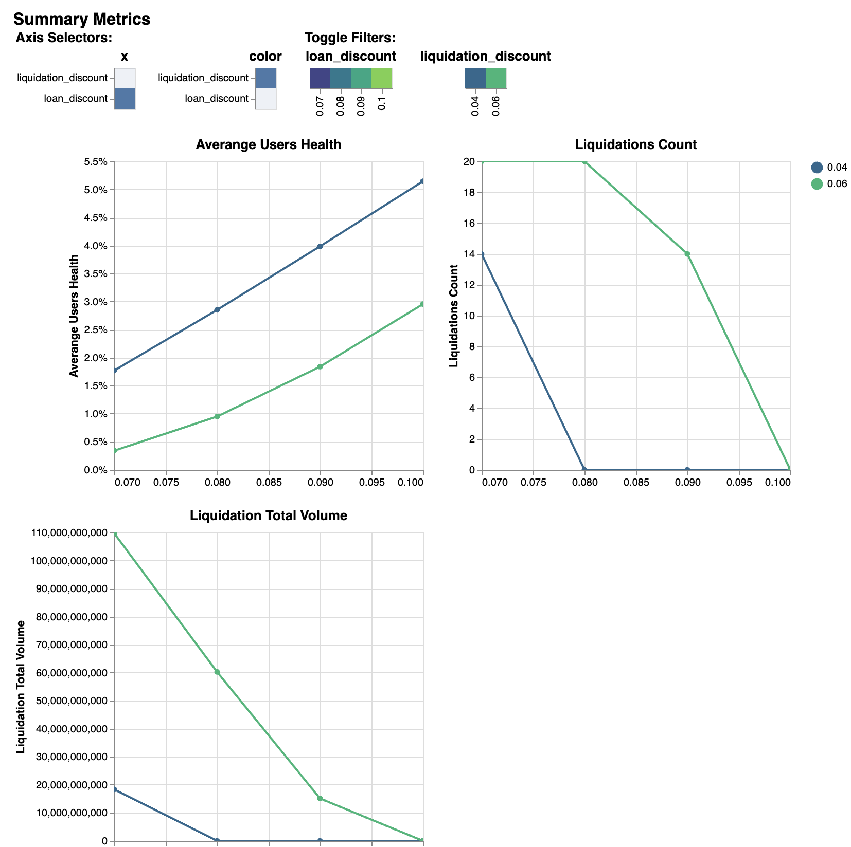
>>> res.summary()
metric averange_user_health liquidations_count liquidation_volume
stat mean max sum
0 0.017705 14.0 1.835876e+10
1 0.003404 20.0 1.097029e+11
2 0.028522 0.0 0.000000e+00
3 0.009494 20.0 6.023163e+10
4 0.039849 0.0 0.000000e+00
5 0.018384 14.0 1.510470e+10
6 0.051448 0.0 0.000000e+00
7 0.029543 0.0 0.000000e+00
>>> res.summary(full=True)
loan_discount liquidation_discount averange_user_health mean liquidations_count max liquidation_volume sum
0 0.07 0.04 0.017705 14.0 1.835876e+10
1 0.07 0.06 0.003404 20.0 1.097029e+11
2 0.08 0.04 0.028522 0.0 0.000000e+00
3 0.08 0.06 0.009494 20.0 6.023163e+10
4 0.09 0.04 0.039849 0.0 0.000000e+00
5 0.09 0.06 0.018384 14.0 1.510470e+10
6 0.10 0.04 0.051448 0.0 0.000000e+00
7 0.10 0.06 0.029543 0.0 0.000000e+00
>>> res.data()
run timestamp averange_user_health liquidations_count liquidation_volume
0 0 2023-09-29 23:30:00+00:00 0.036510 0.0 0.0
1 0 2023-09-29 23:38:34+00:00 0.036509 0.0 0.0
2 0 2023-09-29 23:47:08+00:00 0.036507 0.0 0.0
3 0 2023-09-29 23:55:42+00:00 0.036504 0.0 0.0
4 0 2023-09-30 00:04:17+00:00 0.036500 0.0 0.0
... ... ... ... ... ...
81987 7 2023-11-29 22:55:42+00:00 0.009380 0.0 0.0
81988 7 2023-11-29 23:04:17+00:00 0.009379 0.0 0.0
81989 7 2023-11-29 23:12:51+00:00 0.009379 0.0 0.0
81990 7 2023-11-29 23:21:25+00:00 0.009379 0.0 0.0
81991 7 2023-11-29 23:30:00+00:00 0.009378 0.0 0.0
81992 rows × 5 columns
>>> res.data(full=True)
loan_discount liquidation_discount run timestamp averange_user_health liquidations_count liquidation_volume
0 0.09 0.04 0 2023-09-29 23:30:00+00:00 0.059287 0.0 0.0
1 0.09 0.04 0 2023-09-29 23:38:34+00:00 0.059286 0.0 0.0
2 0.09 0.04 0 2023-09-29 23:47:08+00:00 0.059284 0.0 0.0
3 0.09 0.04 0 2023-09-29 23:55:42+00:00 0.059281 0.0 0.0
4 0.09 0.04 0 2023-09-30 00:04:17+00:00 0.059277 0.0 0.0
... ... ... ... ... ... ... ...
81987 0.12 0.06 7 2023-11-29 22:55:42+00:00 0.032402 0.0 0.0
81988 0.12 0.06 7 2023-11-29 23:04:17+00:00 0.032401 0.0 0.0
81989 0.12 0.06 7 2023-11-29 23:12:51+00:00 0.032401 0.0 0.0
81990 0.12 0.06 7 2023-11-29 23:21:25+00:00 0.032400 0.0 0.0
81991 0.12 0.06 7 2023-11-29 23:30:00+00:00 0.032400 0.0 0.0
81992 rows × 7 columns
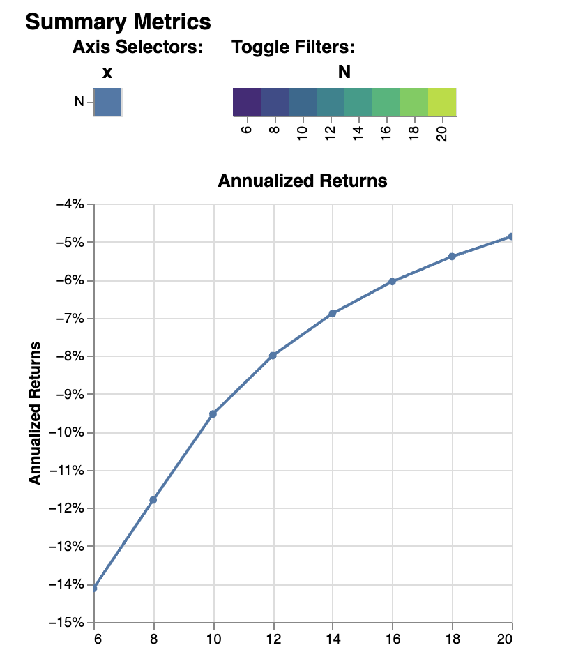
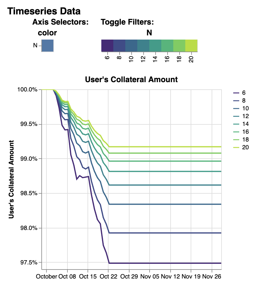
To simlate create_loan with different N parameters, use sim_mode="N":
>>> res = crvusdsim.autosim(pool="wstETH", sim_mode="N", N=[4, 6, 8, 10, 20, 40, 50])

[INFO][17:17:50][crvusdsim.pipelines.simple]-91016: Simulating mode: N
[INFO][17:17:53][curvesim.price_data.sources]-91016: Fetching CoinGecko price data...
[INFO][17:17:59][crvusdsim.templates.Strategy]-91351: [Curve.fi Stablecoin wstETH] Simulating with {'N': 8}
[INFO][17:18:01][crvusdsim.templates.Strategy]-91354: [Curve.fi Stablecoin wstETH] Simulating with {'N': 40}
[INFO][17:18:01][crvusdsim.templates.Strategy]-91349: [Curve.fi Stablecoin wstETH] Simulating with {'N': 4}
[INFO][17:18:01][crvusdsim.templates.Strategy]-91355: [Curve.fi Stablecoin wstETH] Simulating with {'N': 50}
[INFO][17:18:01][crvusdsim.templates.Strategy]-91352: [Curve.fi Stablecoin wstETH] Simulating with {'N': 10}
[INFO][17:18:01][crvusdsim.templates.Strategy]-91353: [Curve.fi Stablecoin wstETH] Simulating with {'N': 20}
[INFO][17:18:01][crvusdsim.templates.Strategy]-91350: [Curve.fi Stablecoin wstETH] Simulating with {'N': 6}

>>> res.summary()

metric      user_value
stat        annualized_returns
0   -0.141162
1   -0.117919
2   -0.095305
3   -0.079963
4   -0.068872
5   -0.060482
6   -0.053912
7   -0.048629

>>> res.summary(full=True)

N   user_value annualized_returns
0   6       -0.141162
1   8       -0.117919
2   10      -0.095305
3   12      -0.079963
4   14      -0.068872
5   16      -0.060482
6   18      -0.053912
7   20      -0.048629

>>> res.data()

    run     timestamp       user_value
0   0       2023-09-29 23:30:00+00:00       1.000000
1   0       2023-09-29 23:38:34+00:00       1.000000
2   0       2023-09-29 23:47:08+00:00       1.000000
3   0       2023-09-29 23:55:42+00:00       1.000000
4   0       2023-09-30 00:04:17+00:00       1.000000
... ...     ...     ...
81987       7       2023-11-29 22:55:42+00:00       0.991699
81988       7       2023-11-29 23:04:17+00:00       0.991699
81989       7       2023-11-29 23:12:51+00:00       0.991699
81990       7       2023-11-29 23:21:25+00:00       0.991699
81991       7       2023-11-29 23:30:00+00:00       0.991699
81992 rows x 3 columns

>>> res.data(full=True)

    N       run     timestamp       user_value
0   6       0       2023-09-29 23:30:00+00:00       1.000000
1   6       0       2023-09-29 23:38:34+00:00       1.000000
2   6       0       2023-09-29 23:47:08+00:00       1.000000
3   6       0       2023-09-29 23:55:42+00:00       1.000000
4   6       0       2023-09-30 00:04:17+00:00       1.000000
... ...     ...     ...     ...
81987       20      7       2023-11-29 22:55:42+00:00       0.991699
81988       20      7       2023-11-29 23:04:17+00:00       0.991699
81989       20      7       2023-11-29 23:12:51+00:00       0.991699
81990       20      7       2023-11-29 23:21:25+00:00       0.991699
81991       20      7       2023-11-29 23:30:00+00:00       0.991699
81992 rows x 4 columns
Results
The simulation returns a SimResults object (here, res) that can plot simulation metrics or return them as DataFrames.
Plotting
The plot() method is used to generate and/or save plots:
#Plot results using Altair
>>> res.plot()

#Save plot results as results_pool.html
>>> res.plot(save_as="results_pool.html")
Screenshots of resulting plots (truncated):
sim_mode="rate"

sim_mode="pool"


sim_mode="controller"
sim_mode="N"
Metrics
The summary method returns metrics summarizing each simulation run:
>>> res.summary()
metric      pool_value      arb_profits_percent     pool_volume     arb_profit      pool_fees
stat        annualized_returns      annualized_arb_profits  sum     sum     sum
0   0.738073        -0.028339       4.828494e+09    8.927715e+06    6.569253e+07
1   0.710731        -0.024171       3.570275e+09    7.637157e+06    8.394951e+07
2   0.750342        -0.028429       4.862393e+09    9.030913e+06    6.623314e+07
3   0.739814        -0.021498       3.466717e+09    6.850344e+06    8.196935e+07
4   0.742118        -0.029061       4.860781e+09    9.280159e+06    6.617865e+07
5   0.727234        -0.023468       3.487223e+09    7.472891e+06    8.250836e+07
6   0.734865        -0.029247       4.905499e+09    9.297305e+06    6.660625e+07
7   0.731708        -0.021982       3.404420e+09    7.003415e+06    8.079451e+07
To include the parameters used in each run, use the full argument:
>>> res.summary(full=True)
    A       Fee     pool_value annualized_returns   arb_profits_percent annualized_arb_profits      pool_volume sum arb_profit sum  pool_fees sum
0   50      0.006   0.738073        -0.028339       4.828494e+09    8.927715e+06    6.569253e+07
1   50      0.010   0.710731        -0.024171       3.570275e+09    7.637157e+06    8.394951e+07
2   60      0.006   0.750342        -0.028429       4.862393e+09    9.030913e+06    6.623314e+07
3   60      0.010   0.739814        -0.021498       3.466717e+09    6.850344e+06    8.196935e+07
4   80      0.006   0.742118        -0.029061       4.860781e+09    9.280159e+06    6.617865e+07
5   80      0.010   0.727234        -0.023468       3.487223e+09    7.472891e+06    8.250836e+07
6   100     0.006   0.734865        -0.029247       4.905499e+09    9.297305e+06    6.660625e+07
7   100     0.010   0.731708        -0.021982       3.404420e+09    7.003415e+06    8.079451e+07
The data method returns metrics recorded at each timestamp of each run:
>>> res.data()
    run     timestamp       pool_value      arb_profits_percent     pool_volume     arb_profit      pool_fees
0   0       2023-09-26 23:30:00+00:00       1.783265e+09    0.000000        0.0     0.0     0.0
1   0       2023-09-26 23:38:34+00:00       1.783349e+09    0.000000        0.0     0.0     0.0
2   0       2023-09-26 23:47:08+00:00       1.783433e+09    0.000000        0.0     0.0     0.0
3   0       2023-09-26 23:55:42+00:00       1.783518e+09    0.000000        0.0     0.0     0.0
4   0       2023-09-27 00:04:17+00:00       1.783602e+09    0.000000        0.0     0.0     0.0
... ...     ...     ...     ...     ...     ...     ...
81987       7       2023-11-26 22:55:42+00:00       1.970115e+09    -0.003708       0.0     0.0     0.0
81988       7       2023-11-26 23:04:17+00:00       1.970115e+09    -0.003708       0.0     0.0     0.0
81989       7       2023-11-26 23:12:51+00:00       1.970115e+09    -0.003708       0.0     0.0     0.0
81990       7       2023-11-26 23:21:25+00:00       1.970115e+09    -0.003708       0.0     0.0     0.0
81991       7       2023-11-26 23:30:00+00:00       1.970115e+09    -0.003708       0.0     0.0     0.0

[81992 rows × 7 columns]
The data method also accepts the full argument. However, the output may be prohibitively large:
>>> res.data(full=True)
    A       Fee     run     timestamp       pool_value      arb_profits_percent     pool_volume     arb_profit      pool_fees
0   50      0.006   0       2023-09-26 23:30:00+00:00       1.783265e+09    0.000000        0.0     0.0     0.0
1   50      0.006   0       2023-09-26 23:38:34+00:00       1.783349e+09    0.000000        0.0     0.0     0.0
2   50      0.006   0       2023-09-26 23:47:08+00:00       1.783433e+09    0.000000        0.0     0.0     0.0
3   50      0.006   0       2023-09-26 23:55:42+00:00       1.783518e+09    0.000000        0.0     0.0     0.0
4   50      0.006   0       2023-09-27 00:04:17+00:00       1.783602e+09    0.000000        0.0     0.0     0.0
... ...     ...     ...     ...     ...     ...     ...     ...     ...
81987       100     0.010   7       2023-11-26 22:55:42+00:00       1.970115e+09    -0.003708       0.0     0.0     0.0
81988       100     0.010   7       2023-11-26 23:04:17+00:00       1.970115e+09    -0.003708       0.0     0.0     0.0
81989       100     0.010   7       2023-11-26 23:12:51+00:00       1.970115e+09    -0.003708       0.0     0.0     0.0
81990       100     0.010   7       2023-11-26 23:21:25+00:00       1.970115e+09    -0.003708       0.0     0.0     0.0
81991       100     0.010   7       2023-11-26 23:30:00+00:00       1.970115e+09    -0.003708       0.0     0.0     0.0

[81992 rows x 9 columns]
Fine-tuning the simulator
Other helpful parameters for autosim() are:
src: data source for prices and volumes. Allowed values are:
“coingecko”: CoinGecko API (free); default
“local”: local data stored in the “data” folder
ncpu: Number of cores to use.
days: Number of days to fetch data for.
end_ts: End timestamp in Unix time.
bands_strategy_class: Strategy used to initialize liquidity in LLAMMA pool bands
1:
class::crvusdsim.pool_data.metadata.BandsStrategy2: valid input:
SimpleUsersBandsStrategy,IinitYBandsStrategy,UserLoansBandsStrategy,3: or a custom strategy that inherits
class::crvusdsim.pool_data.metadata.BandsStrategy
prices_max_interval: The maximum interval for pricing data. If the time interval between twoadjacent data exceeds this value, interpolation processing will be performed automatically.
profit_threshold: Profit threshold for arbitrageurs, trades with profits below this value will not be executed
Tips
Pricing data
By default, crvUSDsim follows the pricing data module of curvesim, uses Coingecko pricing and volume data. To replace the no longer available Nomics service, we expect to onboard another data provider and also provide an option to load data files.
Note on CoinGecko Data
Coingecko price/volume data is computed using all trading pairs for each coin, with volume summed across all pairs. Therefore, market volume taken from CoinGecko can be much higher than that of any specific trading pair used in a simulation. This issue is largely ameloriated by our volume limiting approach, with CoinGecko results typically mirroring results from pairwise data, but it should be noted that CoinGecko data may be less reliable than more granular data for certain simulations.
Parallel processing
By default, crvUSDsim will use the maximum number of cores available to run
simulations. You can specify the exact number through the ncpu option.
For profiling the code, it is recommended to use ncpu=1, as common
profilers (such as cProfile) will not produce accurate results otherwise.
Errors and Exceptions
All exceptions that crvUSDsim explicitly raises inherit from
curvesim.exceptions.curvesimException.